Signal Detection - Cosine Similarity and SNR (2/4)

In the first post on signal detection, we mentioned that a key benefit of using cosine similarity $q$ as a signal detection metric is its direct connection to the Signal-to-Noise Ratio (SNR).

In this note, we state and derive the formula under these two cases :

• xcorr with a clean template
• xcorr with a noisy template

The formula are different and I often had to look it up. Thus the importance of this post to serve as my future reference

Summary

Situation	$q$ –> SNR	SNR –> $q$
xcorr between two noisy signal		$q^2 = \dfrac{\gamma_1}{(1+\gamma_1)} \dfrac{\gamma_2}{(1+\gamma_2)}$
xcorr between two equally noisy signal	$\gamma =\dfrac{q}{1-q}$	$q =\dfrac{\gamma}{1+\gamma}$
xcorr between clean and noisy signal	$\gamma =\dfrac{q^2}{1-q^2}$	$q^2 =\dfrac{\gamma}{1+\gamma}$

Derivation

Notations

Consider two noisy observations of a signal.

\[X_1 = S + N_1\] \[X_2 = S + N_2\]

$S$ is a complex-valued constant vector of length $T$ representing the signal.

$N_1$ and $N_2$ are both complex-valued gaussian noise vectors also of length $T$.

We specify the individual elements of the vector through index $i$. \(X_1[i] = S[i] + N_1 [i]\) \(X_2[i] = S[i] + N_2 [i]\)

For convenience, we define the following symbols to represent power and SNR:

Description	Expression	Symbol
Noise power of $N_1$	$\sum_i[N_1[i] N^*_1[i]]/L$	$\beta_1$
Noise power of $N_2$	$\sum_i[N_2[i] N^*_2[i]]/L$	$\beta_2$
Signal power	$\sum_i[S[i] S^*[i]]/L$	$\alpha$
SNR of $X_1$	$\frac{\alpha}{\beta_1}$	$\gamma_1$
SNR of $X_2$	$\frac{\alpha}{\beta_2}$	$\gamma_2$

Definition of cosine similarity $q$

Cosine Similarity $q$ is a real number

\[\begin{aligned} q &= \frac{|\langle X_1,X_2 \rangle|}{\Vert X_1 \Vert \Vert X_2 \Vert}\\ \end{aligned}\]

$\langle \cdot, \cdot \rangle$ is a inner product between two vectors.

$\Vert \cdot \Vert$ is the L2 norm of the vector.

$ \mid \cdot \mid$ is the absolute value of a complex number.

Both the absolute value and L2 norm operation involves a square root and that is analytically annoying. So we will analyse instead the squared cosine similarity $q^2$.

\[q^2 = \frac{\Vert \langle X_1,X_2 \rangle \Vert^2}{\Vert X_1 \Vert^2 \Vert X_2 \Vert^2}\]

Crunching the Algebra

\(\begin{aligned} \text{Numerator of }q^2 &= \sum_i \Bigl(X_1[i]X^*_2[i]\Bigl) \sum_i \Bigl(X^*_1[i]X_2[i]\Bigl) \\ &= \sum_i \Bigl((S[i] + N_1[i])(S^*[i] + N^*_2[i])\Bigl) \sum_i \Bigl((S^*[i] + N^*_1[i])(S[i] + N_2[i])\Bigl) \\ &= \sum_i \Bigl(S[i]S^*[i] + N_1[i]N_2^*[i] + S[i]N_2^*[i] + S^*[i]N_1[i]\Bigl) \sum_i \Bigl(S[i]S^*[i] + N^*_1[i]N_2[i] + S^*[i]N_2[i] + S[i]N^*_1[i]\Bigl) \\ \end{aligned}\)

Because noise is zero mean, independent and uncorrelated between instances, many terms involving the noise samples average to 0 in the limit of large number of samples $T$.

\[\begin{aligned} \text{Numerator of }q^2 &= \sum_i \Bigl( S[i]S^*[i]\Bigl) \sum_i \Bigl(S[i]S^*[i]\Bigl) \\ &= TT sss^*s^*\\ &= TT\alpha\alpha \end{aligned}\]

As for the denominator

\[\begin{aligned} \text{Denominator of }q^2 &= \sum_i \Bigl(X_1[i] X_1^*[i]\Bigl) \Bigl(X_2[i] X_2^*[i]\Bigl) \\ &= \sum_i \Bigl((S[i] + N_1[i]) (S^*[i] + N_1^*[i])\Bigl) \sum_i \Bigl( (S[i] + N_2[i]) (S^*[i] + N^*_2[i])\Bigl) \\ &= \sum_i \Bigl(S[i]S^*[i] + S^*[i]N_1[i]+ S[i]N_1^*[i] + N_1[i] N_1^*[i] \Bigl) \sum_i \Bigl( S[i]S^*[i] + S^*[i]N_2[i]+ S[i]N_2^*[i] + N_2[i] N_2^*[i]\Bigl) \\ \end{aligned}\]

Similarly, due to the independence of noise

\[\begin{aligned} \text{Denominator of }q^2 &= \sum_i \Bigl(S[i]S^*[i] + N_1[i] N_1^*[i] \Bigl) \sum_i\Bigl(S[i]S^*[i]+ N_2[i] N_2^*[i]\Bigl) \\ &= T \left(\alpha + \beta_1\right) T \left(\alpha + \beta_2\right) \\ &= TT(\alpha + \beta_1) (\alpha + \beta_2) \\ \end{aligned}\]

Putting it all together,

\[\begin{aligned} q^2 &= \frac{TT\alpha\alpha}{TT(\alpha + \beta_1) (\alpha + \beta_2)} \\ &= \frac{\alpha\alpha}{(\alpha + \beta_1) (\alpha + \beta_2)} \\ q^2 &= \dfrac{\gamma_1}{(1+\gamma_1)} \dfrac{\gamma_2}{(1+\gamma_2)}\\ \end{aligned}\]

Results

Case 1: Cosine Similarity between two noisy signals of equal SNR

If noise power was the same for both signals, $\beta_1$ = $\beta_2$ = $\beta$, then SNR of both signals are the same $\gamma_1$ = $\gamma_2$ = $\gamma$

\[\begin{aligned} q^2 &= \left(\frac{\gamma}{1 + \gamma}\right)^2\\ q &= \frac{\gamma}{1 + \gamma}\\ \gamma &= \frac{q}{1-q}\\ \end{aligned}\]

You may simulate this in python to verify the correctness of the formula.

nsamples = 5000
snrdbs = np.linspace(-10,20,400)

def getnoise():
    nn = np.random.randn(2*nsamples).view(np.complex128)
    return nn/np.sqrt(2)

qfs = np.zeros_like(snrdbs)
for i, snrdb in enumerate(snrdbs):
    s = np.sqrt(10**(snrdb/10))
    x1 = s + getnoise()
    x2 = s + getnoise()

    x1 = x1/ np.linalg.norm(x1)
    x2 = x2/ np.linalg.norm(x2)
    qfs[i] = np.abs(np.sum(x1*x2))

plt.figure()
plt.plot(qfs,snrdbs, label="simulated")
plt.plot(qfs,10*np.log10(qfs/(1-qfs)), label="analytical")
plt.xlabel("q")
plt.ylabel("SNR(dB)")
plt.title("Case 1: Cosine Similarity btwn 2 noisy signals")
plt.legend()
plt.grid()
plt.show()

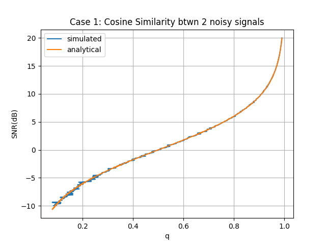
The simulation result matches theory from the high SNR to low SNR regime. Simulation shows greater jitter (variance) at the low SNR regime, but the jitter reduces if the number of samples, $T$, increases.

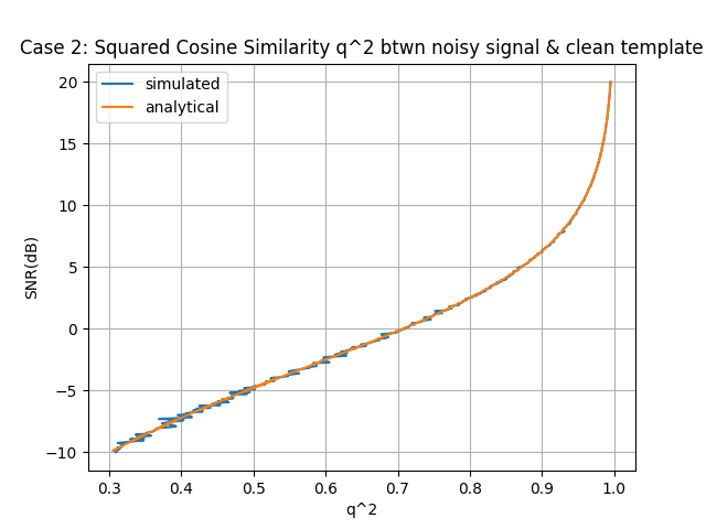
Case 2: Cosine Similarity between a noisy signal and a clean template

Often, we know the signal template and cross-correlating clean template through a noisy signal recording. The height of the cosine similarity peak can actually help us estimate the SNR of the noisy signal.

Setting $\beta_1$ = 0 because the template is noiseless,

\[\begin{align*} q^2 &= \frac{\alpha\alpha}{\alpha(\alpha + \beta_2)}\\ q^2 &= \frac{\alpha}{(\alpha + \beta_2)}\\ q^2 &= \frac{\gamma_2}{1 + \gamma_2}\\ \gamma_2 &= \frac{q^2}{1-q^2}\\ \end{align*}\]

You may simulate this in python to verify the correctness of the formula.

qfs_oneside = np.zeros_like(snrdbs)
for i, snrdb in enumerate(snrdbs):
    snr = 10**(snrdb/10)
    x3 = np.sqrt(snr) + getnoise()
    x4 = np.sqrt(snr) * np.ones(nsamples)

    x3 = x3/ np.linalg.norm(x3)
    x4 = x4/ np.linalg.norm(x4)
    qfs_oneside[i] = np.abs(np.sum(x3*x4))
qf2s_oneside = np.square(qfs_oneside)

plt.figure()
plt.plot(qfs_oneside,snrdbs, label="simulated")
theory = 10*np.log10(qf2s_oneside/(1-qf2s_oneside))
plt.plot(qfs_oneside, theory, label="analytical")
plt.xlabel("q^2")
plt.ylabel("SNR(dB)")
plt.title("Case 2: Squared Cosine Similarity q^2 btwn noisy signal & clean template")
plt.legend()
plt.grid()
plt.show()

Summary

These results show that cosine similarity (or “detection score”) provides a direct connection to SNR. When correlating two noisy observations, the similarity degrades more rapidly compared to correlating with a clean template.