
Signal Detection - Performance of Known Signal Detection (3/4)
In the first post on signal detection, we mentioned that if we know the signal we wish to detect, we can perform two types of cross correlation:
- Matched Filtering with CFAR thresholding
- Cosine Similarity with static thresholding
Which method should we use? Which method is better?
This note analytically derives the performance of each detector as a function of length $L$ and SNR $\gamma$.
Problem Formulation: Hypothesis Testing
A cross correlation based signal detector could be formulated as a sliding classifier. At every sample instance, the classifier chooses between two possible hypotheses:
\[\begin{aligned} \mathcal{H}_0 &: \text{(No signal)} & \underline{y} &= \underline{\eta} \\ \mathcal{H}_1 &: \text{(Signal present)} & \underline{y} &= s\underline{x} + \underline{\eta} \end{aligned}\]where:
- $\underline{y}$ is a complex-valued received signal vector of length $L$
- $\underline{x}$ is a complex-valued signal vector of length $L$
- $\underline{\eta}$ is a complex gaussian noise vector of length $L$
- $s$ is a real valued scalar representing the strength of the signal.
Test statistics
The classifier maps the physical observable $\underline{y}$ into a real valued test statistic $z$ for decision making through thresholding
Matched Filtering’s test statistic :
\[z_{mf} = \frac{|\langle \underline{y}, \underline{x} \rangle|^2}{L}\]Cosine Similarity’s test statistic:
\[z_{cs} = \frac{|\langle \underline{y}, \underline{x} \rangle|^2}{\Vert \underline{y} \Vert^2 \Vert \underline{x} \Vert^2}\]Where:
- $ | \cdot | $ refers to absolute value of a complex-valued scalar
- $\Vert \cdot \Vert $ refers to the L2 norm of a complex valued vector
- $\underline{y}$ and $\underline{x}$ are vectors of length $L$
Additional Assumptions
To ease the analysis of these test statistics, we assume the following:
- every element in vector $\underline{x}$ is unit modulus
- every element in $\underline{\eta}$ is an independent standard complex random gaussian with unit variance in its real and imaginary parts
Thus the energy of signal $\underline{x}$ is $Ls^2$, and the energy of the noise $\underline{\eta}$ is $2L$. Signal to Noise Ratio $\gamma$ is then
\[\text{SNR} = \gamma = \frac{s^2}{2}\]Often it is more practical to parameterize this problem using SNR $\gamma$ because it is unitless. So
\[\begin{aligned} \mathcal{H}_0 &: \text{(No signal)} & \underline{y} &= \underline{\eta} \\ \mathcal{H}_1 &: \text{(Signal present)} & \underline{y} &= \sqrt{2\gamma}\underline{x} + \underline{\eta} \end{aligned}\]Summary
| Hypothesis | Distribution of $z_{mf}$ | Distribution of $z_{cs}$ |
|---|---|---|
| $\mathcal{H}_0$ : No Signal | $\mathcal{X}^2(k=2)$ | $Beta(a=1,b=L-1)$ |
| $\mathcal{H}_1$ : Signal Present | $\chi_{nc}^2(k=2, \lambda=2L\gamma)$ | $Beta_{nc}(a=1,b=L-1, \lambda=2L\gamma)$ |
Visualization of distribution
Matched Filter test statistic $z_{mf}$
Cosine Similarity test statistic $z_{cs}$
As SNR $\gamma$ increases, so does the separation between the blue $\mathcal{H}_0$ distribution and yellow $\mathcal{H}_1$ distribution, thus increasing the ease of correctly classifying between both hypotheses and thus detecting the signal.
As $L$ increases, the separation between both distributions also increases due to the integration gain effect
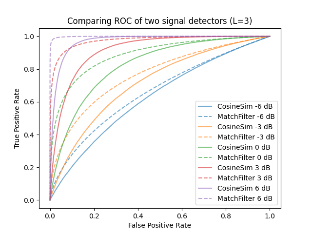
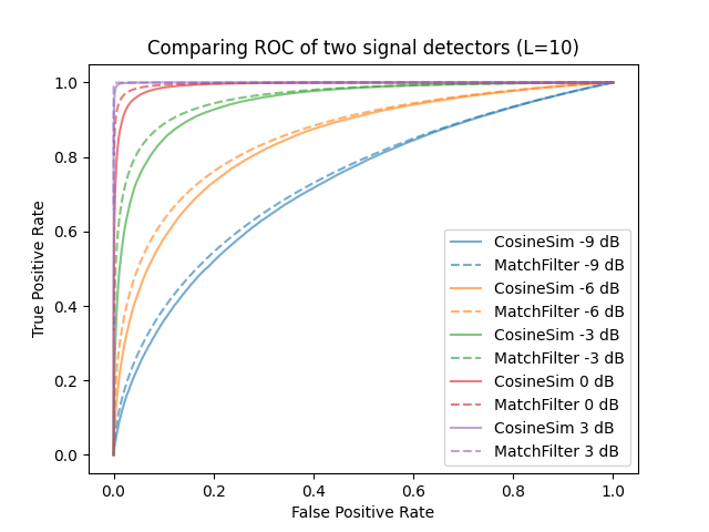
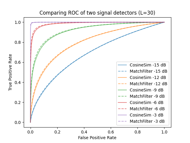
Receiver Operator Curves
For a signal of fixed length $L$ and SNR $\gamma$, varying the decision threshold on $z_{mf}$ can only tradeoffs between the probability of detection (Pd) and the probability of false alarm (Pfa). In other words, the quality of the classifier is determined by the test statistic and not the threshold.
This leads to the concept of a receiver operator curve which plots the Pd and Pfa for every threshold. The greater the area under curve, the better the classifier.
Derivation of Matched Filter test statistic $z_{mf}$ distribution
$\mathcal{H}_0$ case: No signal present
\[\begin{align*} z_{mf} &= |\langle \underline{y}, \underline{x} \rangle|^2 /L\\ &= \left| \sum_{i=1}^L (\underline{\eta}[i] * \underline{x}^*[i]) \right|^2 / L\\ &= \left| \sum_{i=1}^L \underline{\eta}'[i] \right|^2 / L \tag{Note 1}\\ &= \left| \eta'' \right|^2 / L \tag{Note 2} \\ &= \left[ \mathcal{N}_{real}\left(0,L\right)^2 + \mathcal{N}_{imag}\left(0,L\right)^2 \right] / L \\ &= \left( \mathcal{N}_{real}\right)^2 + \left( \mathcal{N}_{imag}\right)^2 \\ \end{align*}\]Explanatory Notes:
- $\underline{\eta}’$ is a vector of random complex gaussian. Its elements differ only in phase from those of $\underline{\eta}$ because the elements of $\underline{x}$ are unit modulus.
- $\eta’’$ is a random complex gaussian scalar with variance $L$ in its real and imaginary.
The sum of two squared gaussians is a chi-square distribution with 2 degrees of freedom and also an exponential distribution with inverse scale parameter $\lambda=1/2$. So
\[\mathcal{H}_0 : \boxed{ z_{mf} \sim \mathcal{X}_2^2\\ }\]or
\[\mathcal{H}_0 : \boxed{z_{mf}\sim Exp(\lambda=1/2)}\]$\mathcal{H}_1$ case: Signal is present
\[\begin{align*} z_{mf} &= |\langle \underline{y}, \underline{x} \rangle|^2 / L\\ &= \left| \sum_{i=1}^L \left(\left(\sqrt{2\gamma}\underline{x}[i] + \underline{\eta}[i]\right) * \underline{x}^*[i]\right) \right|^2 / L\\ &= \left| \sum_{i=1}^L \left(\sqrt{2\gamma} + \underline{\eta}'[i]\right) \right|^2 / L \\ &= \left| L\sqrt{2\gamma} + \eta'' \right|^2 / L \\ &= \left[ \mathcal{N}_{real}(L\sqrt{2\gamma},L)^2 + \mathcal{N}_{imag}(0,L)^2 \right] / L \\ &= \left(\mathcal{N}_{real} (\sqrt{2\gamma L} ,1 )\right)^2 + \left( \mathcal{N}_{imag} \right)^2 \\ \end{align*}\]The sum of two squared gaussians whose mean may be non-zero is a non-central chi-squared distrbution. Here, the degree of freedom $k= 2$ and noncentrality parameter $\lambda = 2\gamma L$
\[\mathcal{H}_1 : \boxed{z_{mf} \sim \chi_{nc}^2(k=2, \lambda=2L\gamma)} \\\]Derivation of cosine similarity test statistic $z_{cs}$ distribution
$\mathcal{H}_0$ case: No signal present
Numerator
First we analyse the numerator:
\[\begin{align*} \text{Numerator of } z_{cs} &= |\langle \underline{y}, \underline{x} \rangle|^2 \\ &= \left| \sum_{i=1}^L (\underline{\eta}[i] * \underline{x}^*[i]) \right|^2 \\ &= \left| \sum_{i=1}^L \underline{\eta}'[i] \right|^2 \\ &= \left| \eta'' \right|^2 \\ &= \left(\mathcal{N}_{real}\left(0,L \right) \right)^2 + \left(\mathcal{N}_{imag}\left(0,L\right) \right)^2 \\ &= L\left[\left(\mathcal{N}_{real} \right)^2 + \left(\mathcal{N}_{imag} \right)^2 \right]\\ \\ \text{Numerator of } z_{cs}&\sim L \chi_2^2 \end{align*}\]Denominator
Now we analyse the denominator:
\[\begin{align*} \text{Denominator of } z_{cs} &= \Vert \underline{y} \Vert^2 \Vert \underline{x} \Vert^2\\ &= \left( \sum_{i=1}^L \left| \underline{\eta}[i] \right|^2 \right) \left( \sum_{i=1}^L \left| \underline{x}[i] \right| ^2 \right) \\ &= L \left( \sum_{i=1}^L \left| \underline{\eta}[i] \right|^2 \right)\\ &= L \left[ \mathcal{N}_{real1}^2 + \dots + \mathcal{N}_{realL}^2 + \mathcal{N}_{imag1}^2 + \dots + \mathcal{N}_{imagL}^2 \right]\\ \\ \text{Denominator of } z_{cs} &\sim L \chi_{2L}^2 \end{align*}\]Wrong Results
Though $z_{cs}$ as a ratio of two chi-squared distributions, it is not F-distributed as the numerator and denominator are not independent random variables.
\[z_{cs} \sim \frac{L \chi_2^2}{L \chi_{2L}^2} = \frac{\chi_2^2}{\chi_{2L}^2} \neq \frac{1}{L}\mathcal{F}(2,2L)\]Change of basis
Fortunately the Beta distribution has a construction similar to the definition of $z_{cs}$:
\[\begin{align*} Beta\left(\frac{k_1}{2},\frac{k_2}{2} \right) &\sim \frac{X}{X+Y} \\ \text{where}\\ X &\sim \chi^2_{k_1}\\ Y &\sim \chi^2_{k_2}\\ \end{align*}\]We can show that $z_{cs}$ is Beta distributed through a change of basis.
First, let’s express $\underline{\eta}$ as a vector of $2L$ real-valued gaussians instead of $L$ complex-valued gaussians
\[\begin{align*} \underline{\eta} &= (\mathcal{CN}_1 \dots \mathcal{CN}_L) \\ &= (\underbrace{\mathcal{N}_1 \dots \mathcal{N}_L}_{\text{real part}}, \underbrace{\mathcal{N}_{L+1} \dots \mathcal{N}_{2L}}_{\text{imag part}}) \end{align*}\]Consider two orthonormal basis:
\[\begin{align*} \underline{e_1} &= \frac{1}{\sqrt{L}}(\underbrace{1,\dots,1}_{L},\underbrace{0,\dots,0}_{L}) \\ \underline{e}_{L+1} &= \frac{1}{\sqrt{L}}(\underbrace{0,\dots,0}_{L},\underbrace{1,\dots,1}_{L}) \\ \end{align*}\]The rest of the basis vectors $\underline{e_2} \dots \underline{e_{L}}$ and $\underline{e}{L+2} \dots \underline{e{2L}}$ in this basis set can be found through Gram–Schmidt process. Alternatively, if $L$ is a power of 2, the basis set can be elegantly constructed from the Hadamard matrix. For example if $L=4$, the coordinate transform matrix could be:
\[\frac{1}{\sqrt{L}} \begin{bmatrix} 1 & 1 & 1 & 1 & 0 & 0 & 0 & 0 \\ 1 & 1 & -1 & -1 & 0 & 0 & 0 & 0 \\ 1 & -1 & -1 & 1 & 0 & 0 & 0 & 0 \\ 1 & -1 & 1 & -1 & 0 & 0 & 0 & 0 \\ 0 & 0 & 0 & 0 & 1 & 1 & 1 & 1 \\ 0 & 0 & 0 & 0 & 1 & 1 & -1 & -1 \\ 0 & 0 & 0 & 0 & 1 & -1 & -1 & 1 \\ 0 & 0 & 0 & 0 & 1 & -1 & 1 & -1 \\ \end{bmatrix}\]The numerator of $z_{cs}$ can be reexpressed as: \(\begin{align*} \text{numerator of } z_{cs} &= \left| \sum_{i=1}^L \underline{\eta}'[i] \right|^2 \\ &= \left(\sqrt{L}\underline{e_1}\cdot \underline{\eta}'\right)^2 + \left(\sqrt{L}\underline{e}_{L+1}\cdot \underline{\eta}'\right)^2 \\ &= L \left[\mathcal{N}^2_1 + \mathcal{N}^2_{L+1} \right] \\ &= L \chi_2^2 \end{align*}\)
The denominator of $z_{cs}$ can be reexpressed as: \(\begin{align*} \text{denominator of } z_{cs} &= L \left( \sum_{i=1}^L \left| \underline{\eta}[i] \right|^2 \right)\\ &= L \left( \sum_{i=1}^{2L} \left( \underline{e_i} \cdot \underline{\eta} \right)^2 \right)\\ &= L \left[ \sum_{i=1}^{2L} \mathcal{N}^2_i\right]\\ \end{align*}\)
Putting numerator and denominator together:
\[z_{cs} = \frac{\mathcal{N}^2_1 + \mathcal{N}^2_{L+1} }{\mathcal{N}^2_1 + \mathcal{N}^2_2 + \dots + \mathcal{N}^2_{2L} } = \frac{\mathcal{X}^2_2}{\mathcal{X}^2_2 + \mathcal{X}^2_{2L-2}}\] \[z_{cs} \sim Beta(1,L-1)\]$\mathcal{H}_1$ case: signal is present
Before Change of Basis
First we analyse the numerator and denominator before change of basis
\[\begin{align*} \text{Numerator of } z_{cs} &= |\langle \underline{y}, \underline{x} \rangle|^2 \\ &= \left| \sum_{i=1}^L \left( \left( \sqrt{2\gamma}\underline{x}[i] + \underline{\eta}[i] \right) \underline{x}^*[i] \right) \right|^2 \\ &= \left| \sum_{i=1}^L \left( \sqrt{2\gamma} + \underline{\eta}'[i] \right) \right|^2 \\ &= \left( \mathcal{N}\left(L\sqrt{2\gamma}, L\right) \right)^2 + \left( \mathcal{N}\left(0,L\right) \right)^2\\ &= L \mathcal{X}_{nc}^2(2,2L\gamma)\\ \end{align*}\]The numerator of $z_{cs}$ is non-central chi-squared distrbuted with degree of freedom $k=2$ and noncentrality parameter $\lambda = 2L\gamma$.
\[\begin{align*} \text{Denominator of } z_{cs} &= \Vert \underline{y} \Vert^2 \Vert \underline{x} \Vert^2 \\ &= \left( \sum_{i=1}^L \left| \sqrt{2\gamma}x[i]+\underline{\eta}[i] \right|^2 \right) \left( \sum_{i=1}^L \left| \underline{x}[i] \right| ^2 \right) \\ &= L \left( \sum_{i=1}^L \left| \sqrt{2\gamma}+\underline{\eta'}[i] \right|^2 \right)\\ &= L \sum_{i=1}^L \left| \mathcal{N}_i(\sqrt{2\gamma}, L) \right|^2 + L \sum_{i=1}^L \left| \mathcal{N}_i(0, L) \right|^2 \\ &= L \mathcal{X}_{nc}^2(2L,2L\gamma)\\ \end{align*}\]The denominator of $z_{cs}$ is non-central chi-squared distrbuted with degree of freedom $k=2L$ and noncentrality parameter $\lambda = 2L\gamma$.
While $z_{cs}$ is a ratio between two non-central chi-squared distributions, the numerator and denominator are not independent. It may also look similar to the definition of the non-central F-distribution but it is not because only the numerator of the non-central F-distribution is non-central.
\[z_{cs} = \frac{\mathcal{X}^2_{nc}(2,2L\gamma)}{\mathcal{X}^2_{nc}(2L,2L\gamma)} \neq \mathcal{F}\]Change of Basis
We have to use the change of basis trick again. This time, the real part of each element in $\eta’$ has a non-zero mean. The change of basis helpfully moves all the mean offset to a single element. Here is an illustration.
\[\frac{1}{\sqrt{L}} \begin{bmatrix} 1 & 1 & 1 & 1 & 0 & 0 & 0 & 0 \\ 1 & 1 & -1 & -1 & 0 & 0 & 0 & 0 \\ 1 & -1 & -1 & 1 & 0 & 0 & 0 & 0 \\ 1 & -1 & 1 & -1 & 0 & 0 & 0 & 0 \\ 0 & 0 & 0 & 0 & 1 & 1 & 1 & 1 \\ 0 & 0 & 0 & 0 & 1 & 1 & -1 & -1 \\ 0 & 0 & 0 & 0 & 1 & -1 & -1 & 1 \\ 0 & 0 & 0 & 0 & 1 & -1 & 1 & -1 \\ \end{bmatrix} \underbrace{ \begin{bmatrix} \mathcal{N}(\sqrt{2\gamma},1) \\ \mathcal{N}(\sqrt{2\gamma},1) \\ \mathcal{N}(\sqrt{2\gamma},1) \\ \mathcal{N}(\sqrt{2\gamma},1) \\ \mathcal{N}(0,1) \\ \mathcal{N}(0,1) \\ \mathcal{N}(0,1) \\ \mathcal{N}(0,1) \\ \end{bmatrix} }_{\sqrt{2\gamma} + \eta'} = \begin{bmatrix} \mathcal{N}(\sqrt{2L\gamma},1) \\ \mathcal{N}(0,1) \\ \mathcal{N}(0,1) \\ \mathcal{N}(0,1) \\ \mathcal{N}(0,1) \\ \mathcal{N}(0,1) \\ \mathcal{N}(0,1) \\ \mathcal{N}(0,1) \\ \end{bmatrix}\] \[\begin{align*} \text{Numerator of } z_{cs} &= \left| \sum_{i=1}^L \left( \sqrt{2\gamma} + \underline{\eta}'[i] \right) \right|^2 \\ &= \left( \sqrt{L}\underline{e_1} \cdot \left( \sqrt{2\gamma} + \underline{\eta}' \right) \right)^2 + \left( \sqrt{L}\underline{e}_{L+1}\cdot \underline{\eta}' \right)^2 \\ &= \left(\mathcal{N}_1(L\sqrt{2\gamma},L)\right)^2 + \left(\mathcal{N}_{L+1}(0,L) \right)^2\\ &= L \left[\left(\mathcal{N}_1(\sqrt{2L\gamma},1)\right)^2 + \mathcal{N}^2_{L+1} \right] \\ \end{align*}\] \[\begin{align*} \text{Denominator of } z_{cs} &= L \left( \sum_{i=1}^L \left|\sqrt{2\gamma}+\underline{\eta'}[i] \right|^2 \right)\\ &= L \left( \sum_{i=1}^{2L} \left( \underline{e_i} \cdot (\sqrt{2\gamma} + \underline{\eta}') \right)^2 \right)\\ &= L \left[ \left(\mathcal{N}_1(\sqrt{2L\gamma}, 1 )\right)^2 + \sum_{i=2}^{2L} \left(\mathcal{N}_i(0, 1 )\right)^2 \right]\\ &= L \left( \left(\mathcal{N}_1(\sqrt{2L\gamma}, 1) \right)^2 + \sum_{i=2}^{2L} \mathcal{N}_i ^2 \right) \\ \end{align*}\]Results
This time, we use the definition of the non-central Beta Distribution
\[NonCentralBeta(\frac{m}{2}, \frac{n}{2}, \lambda) = \frac{\mathcal{X}^2_{nc}(m, \lambda)}{\mathcal{X}^2_{nc}(m, \lambda) + \mathcal{X}^2_n}\] \[z_{cs} = \frac{\mathcal{N}^2_1 + \mathcal{N}^2_{L+1} }{\mathcal{N}^2_1 + \mathcal{N}^2_2 + \dots + \mathcal{N}^2_{2L} } = \frac{\mathcal{X}^2_{nc}(2,2L\gamma)}{\mathcal{X}^2_{nc}(2,2L\gamma) + \mathcal{X}^2_{2L-2}}\] \[z_{cs} \sim NonCentralBeta(1,L-1, 2L\gamma)\]