Signal Detection - Introduction (1/4)

Signal detection is a fundamental problem in signal processing, encountered in applications ranging from radar and communications to biomedical systems. The objective is to determine whether a signal of interest is present within noisy observations. Because detection is both conceptually simple and practically important, a wide variety of methods have been developed—ranging from heuristic thresholding techniques to approaches with firm statistical foundations.

This note consolidates several basic detection strategies, with an emphasis on practical, intuitive methods. To motivate the discussion, we consider the following scenario.

Problem: Signal Detection

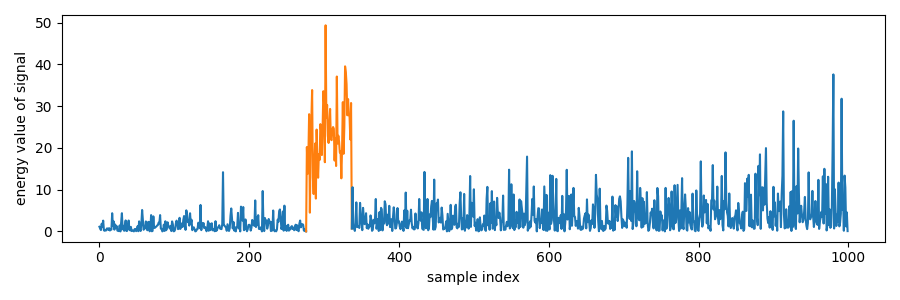
Suppose we observe a time series containing a burst of a complex-valued signal embedded in complex-valued Gaussian noise. Unlike the idealized case of stationary noise, the noise power here varies over time, creating a fluctuating noise floor. The task is to detect the presence and extent of the signal burst.

Static thresholding

A straightforward approach is to apply a static threshold to the signal energy. If the instantaneous energy exceeds the threshold, the corresponding sample is declared as part of the signal burst. While simple and fast, this method may miss weaker portions of the burst that fall below the threshold.

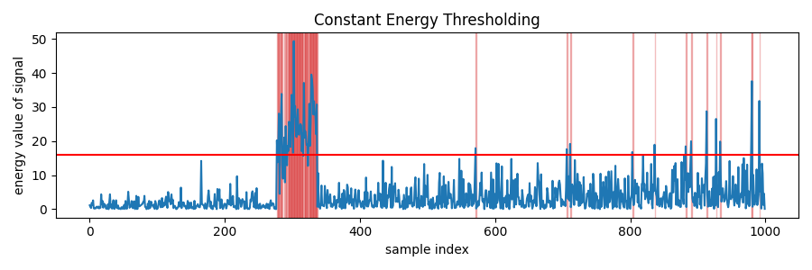
Static thresholding on the instantaneous samples of raw time series may also result in gaps when the instantanous magnitude dips below the threshold. To detect the continuous extent of the signal burst, two common heuristics could be employed.

Hysteresis Detection

In hystersis detection, there are two static thresholds. The sample need to rise above the upper threshold to detect the start the burst and the sample need to fall below the lower threshold to detect the end of the burst. Hysteresis thresholding is sometimes called “edge detection”.

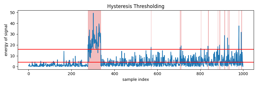
As can be seen in the figure above, the entire signal burst is detected as one segment. Due to the increasing noise floor, we also got some false alarms in the later part of the time series.

Hysteresis a viable method to detect radar signals as radar bursts often have constant power. But burst communications RF bursts may legitimately have instantaneous samples which dips to zero. This makes setting the lower threshold impossible. So instead, morphological operations can be used to directly clean up the breaks between the detections.

Morphological Post-processing

Morphological operations work on binary arrays. For our application, we performed binary closing first to close up any breaks smaller than 5 samples long in the detected signal. Afterwards, we performed binary opening to remove any detected segments shorter than 5 samples long. 5 samples is just an heuristic choice of parameter. We can use other parameters for other applications.

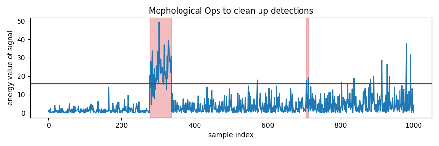
As can be seen in the figure above, there are fewer false alarms. We could have removed that false alarm had we performed binary opening with structure size greater than 5.

The structure size of the morphological operation is empirically determined.

Method 2: Dynamic Threshold (CFAR)

Static thresholds do not adapt to a changing noise floor. Even in environments with stationary noise, different receivers may introduce varying gain levels, making it inconvenient to manually set a fixed threshold. A more robust strategy is to adjust the threshold dynamically as a function of the estimated noise level.

The Constant False Alarm Rate (CFAR) detector accomplishes this by scaling the estimated noise power with a fixed multiplier. For instance, one might set the threshold at 5x the estimated noise power. This ensures that the probability of false alarm remains consistent across different noise conditions.

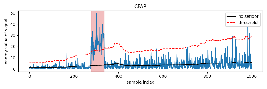
Estimating noise floor

The challenge lies in estimating the noise floor without contamination from the signal itself. Since this is not possible directly, the estimate must rely on portions of the data assumed to contain only noise. A sliding window approach is commonly employed:

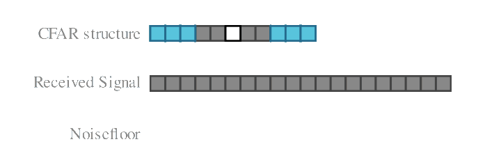
• Guard samples adjacent to the test cell are excluded to prevent signal leakage into the estimate.
• Reference samples further away are averaged to estimate the noise power.

The length of the guard region should be at least as large as the expected signal burst, while the number of reference samples balances estimation accuracy against the assumption of burst spacing.

Lazy alternative

Now, I am often lazy and it is a bit tedious to construct such a window in python to correlate. So I often simply use scipy's median_filter to estimate the noisefloor and ensure that my window is at least 3x the size of the burst. I may sometimes divide the median filter's output by $log(2)$ to convert the median into a mean.

Constant False Alarm Rate Property

To understand why CFAR achieves a constant false alarm probability, consider a complex Gaussian noise sample \(x = a + ib,\quad a,b \sim \mathcal{N}(0, \sigma^2).\)

The instantaneous energy is distributed as \(|x|^2 = a^2 + b^2 \sim \text{Exponential}!\left(\lambda = \tfrac{1}{2\sigma^2}\right).\)

Note that $ |x| ^2$ is sometimes stated as chi-squared distributed with degree 2. This is also correct as a chi-squared distribution with $k=2$ is a scaled exponential distribution.

The mean and standard deviation of this exponential distribution are both $2\sigma^2$. If the threshold is set to $m$ times the mean, the false alarm probability becomes

\[P_{FA} = \Pr{|x|^2 > m \cdot \mathbb{E}[|x|^2]} = e^{-m}.\]

This expression is independent of $\sigma$, demonstrating the “constant” false alarm rate property. For example, with $m = 5$, the expected fraction of false alarms is $e^{-5} \approx 0.0067$.

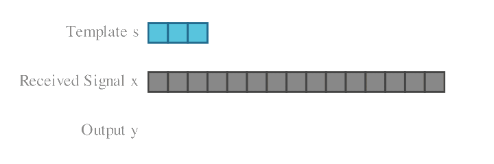
Method 3: Matched Filter + CFAR

When the signal of interest is known, detection performance can be improved by correlating the received sequence with a reference template. In Radar signal processing literature, this operation is referred to as matched filtering or pulse compression .

Formally, the matched filter output is given by

\[y[t] = \sum_i s^*[i],x[t+i],\]

where $s$ is the known signal. The conjugation ensures that contributions from the signal add coherently, while noise accumulates incoherently. The result is an integration gain proportional to the signal length, enabling the detection of weak signals.

The output of the matched filter coherently compresses (thus the name) the entire burst into a prominent peak. Consequently, instead of detecting burst start and end points, the detector only needs to identify the correlation peak.

Because the signal of interest was summed in a phase coherent manner and the noise was summed incoherently, signals that were buried and seemingly undetectable under the noise floor could rise up as a prominant peak post matched filtering. This apparent increase in Signal to Noise Ratio (SNR) is attributed to the “integration gain” of the matched filtering operation and is proportional to the bandwidth time product of the signal.

Integration Gain $= 10*\log_{10}(\text{bandwidth time product of signal})$

So if the signal of length (100 samples) had a 3dB SNR before matched filtering, it would appear to have a 23dB SNR correlation peak post matched filtering. Matched filtering allows the detection of very weak signal buried under the noisefloor.

However, the matched filter output still scales with the noise floor. Therefore, a CFAR threshold is typically applied to the matched filter output to maintain robustness. The correlation window also produces sidelobes (“skirting”) around the peak, necessitating guard regions at least as long as the signal burst.

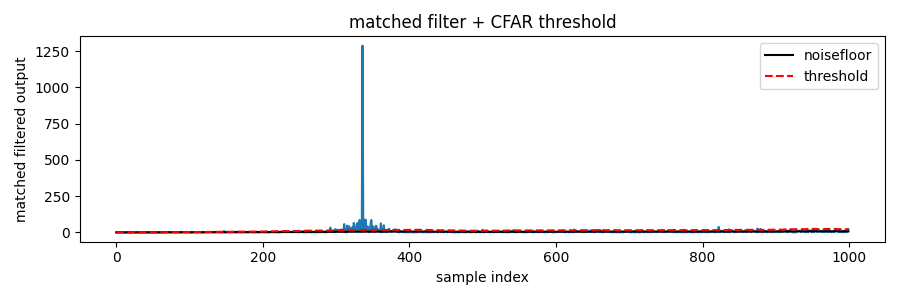
Notice also that around the peak there is a “skirting”. This skirting is due to our correlation window entering and exiting the signal region. So even though we have “compressed” the burst into a single peak, the CFAR guard samples still needs to be as long as the burst length itself.

Method 4: Cosine Similarity

CFAR assumes that the reference samples adjacent to the test cell are free of signal. In scenarios where this assumption does not hold, an alternative approach is to normalize the correlation with respect to signal and noise energy, leading to a cosine similarity detector.

\[q[t] = \frac{\langle x_t,s \rangle}{\Vert x_t \Vert \Vert s \Vert} = \frac{\sum_i s^*[i]x[t+i]}{\Vert x_t \Vert \Vert s \Vert}\\\]

• $\langle \cdot, \cdot \rangle$ is a inner product between two vectors.
• $\Vert \cdot \Vert$ is the L2 norm of the vector.
• $x_t$ is a segment of the received signal of the same length as the template $s$ and starting at index $t$

Note that different authors may refer to this quantity by different names. For instance, Eduardo calls it the detection score. We however adopted the term cosine similarity, as the concept of cosine similarity is increasingly well-known due to its use in vector databases and machine learning.

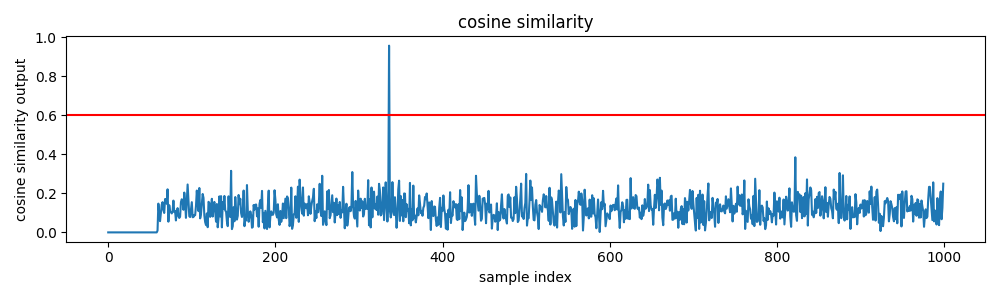
The magnitude of $q[t]$ lies between 0 and 1, independent of the absolute signal or noise power. This normalization makes threshold selection more straightforward and interpretable. In particular, the relationship

\[|q|^2 = \frac{\text{SNR}}{1+\text{SNR}}\]

connects the cosine similarity threshold directly to the minimum detectable SNR. For instance, requiring $

q

^2 > 0.5$ implicitly corresponds to detecting signals with SNR greater than 1 (0 dB).

Moreover, cosine similarity preserves the constant false alarm rate property, although the exact distribution of the normalized correlation follows a generalized F-distribution, making closed-form expressions less convenient. Nonetheless, the invariance to noise power ensures consistent detection performance.